Contamination Bias in Linear Regressions
Economists love using linear regression to estimate treatment effects — it turns out that there are perils to this method, but also amazing perks. [-0-] [-0-] This post is a synthesis of a Twitter/Bluesky thread.
In this post, I’ll discuss how…
- Some of the problems with linear regressions in the recent TWFE/DiD lit generalize to other strategies.
- Regression can be best for estimating treatment effects when these problems aren’t present.
- To bring back regression’s mojo when the problems exist.
High-level intuition
To understand this, we need to really understand what’s going on when we use linear regression to estimate a treatment effect when we have both:
- Heterogeneous effects
- Controls
Consider a simple example: an randomized control trial (RCT) of a binary intervention $D$ on outcome $Y$, where the intervention $D$ is random conditional on a binary control $W$ (e.g., the propensity score is not the same across $W$).
\[(Y(1), Y(0)) \perp D \; \vert \; W\]To estimate the effect of the intervention, many economists would run the regression of:
\[Y = \alpha + \beta D + \gamma W + \varepsilon\]And report the coefficient on $D$, $\beta$, confident that it’s a convex combination of treatment effects $\tau(w) = E(Y(1) - Y(0) \vert W=w)$, thanks to Angrist (1998) and Mostly Harmless Econometrics. [-1-] [-1-] Angrist (1998) showed that regression coefficients like $\beta$ identify a convexly-weighted average of within-strata ATEs for a single binary control $W$. Mostly Harmless Econometrics generalized this to multivalued controls, but still focus on binary treatments. Formally, this result looks like:
\[\beta=\phi\tau_{1}(0)+(1-\phi)\tau_{1}(1)\]where
\[\phi= \frac{Var(D_i\mid W_i=0)\Pr(W_i=0)}{\sum_{w=0}^{1} Var(D_i\mid W_i=w)\Pr(W_i=w)}\in [0,1].\]This result shows how regression avoids some problems of other estimation procedures (e.g., inverse pscore weighting): namely infeasibility or imprecision when the propensity score $p(w) = E(D \vert W = w)$ is extreme. The regression estimate automatically puts less weight on such values of W. This is the ideal case, where we know that we can estimate the causal effect of D on Y!
Our paper (with Peter Hull and Michal Kolesár) shows three things:
- This automatic variance weighting gives the estimator that is “easiest” to estimate in the binary treatment case (using OLS achieves a semiparametric bound under homoskedasticity). Basically, OLS picks weights across covariate groups to maximize the variation in the treatment!
- This automatic variance weighting intuition doesn’t generalize to multiple correlated treatments (which includes multi-armed RCTs, and staggered diff-in-diff!), and can create contamination bias across treatment estimates, even when you have zero omitted variable bias (!) [-2-] [-2-] What we call contamination bias is effectively a spillover of the other treatments into either the control or treatment group for the treatment of interest. .
- We show how you can fix the contamination bias with an estimator which again gives the automatic variance weighting. We also provide a Stata package and an R package to implement this estimator (and also check for contamination bias).
Unpacking this further
Let’s try to unpack what’s going on, and along the way, we can learn new things about estimation with heterogeneous treatment effects and how the difference between design-based identification and model-based identification can lead to different regression weights.
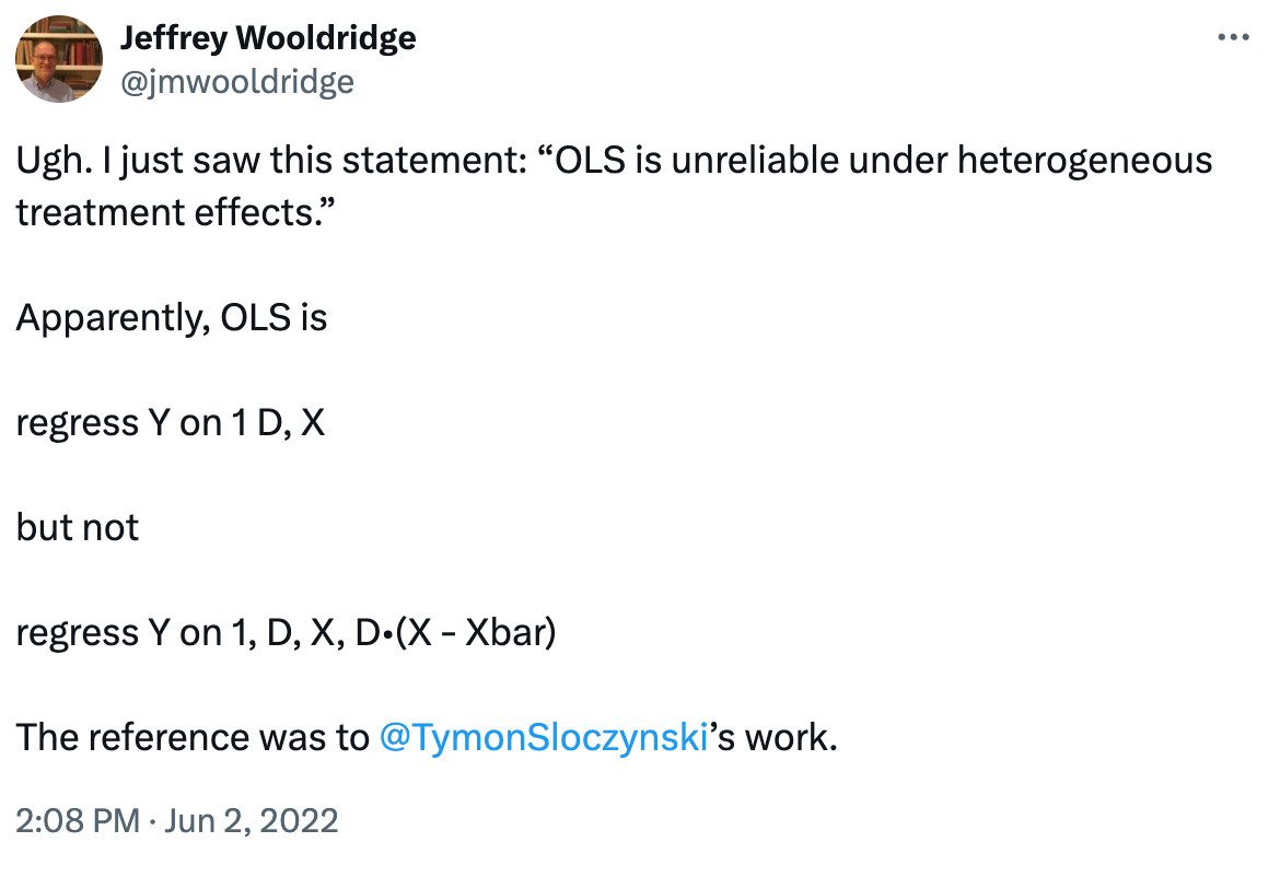
First, note that regression can provide you with the ATE, rather than the variance weighted effect, as Jeff Wooldridge alludes to in this tweet. The solution is straightforward – by interacting the demeaned control $W$ with $D$:
\[Y_{i} = \alpha + D_i'\beta + W_i'\gamma + D_{i}(W_i -E(W_i))\delta + \varepsilon_i\]In this regression, the coefficient on $D_{i}$, $\beta$, will recover the ATE! However, this makes OLS susceptible to the same imprecision concerns as propensity score weighting. This solution will be important going forward.
Now, imagine now that $D$ can be two treatments: $D \in {0,1,2}$.
The natural extension of our original regression is
\[Y = \alpha + \beta_{1} X_1 + \beta_2 X_2 + \gamma W + \varepsilon\]Where the $X$ are dummies for $D =1,2$.
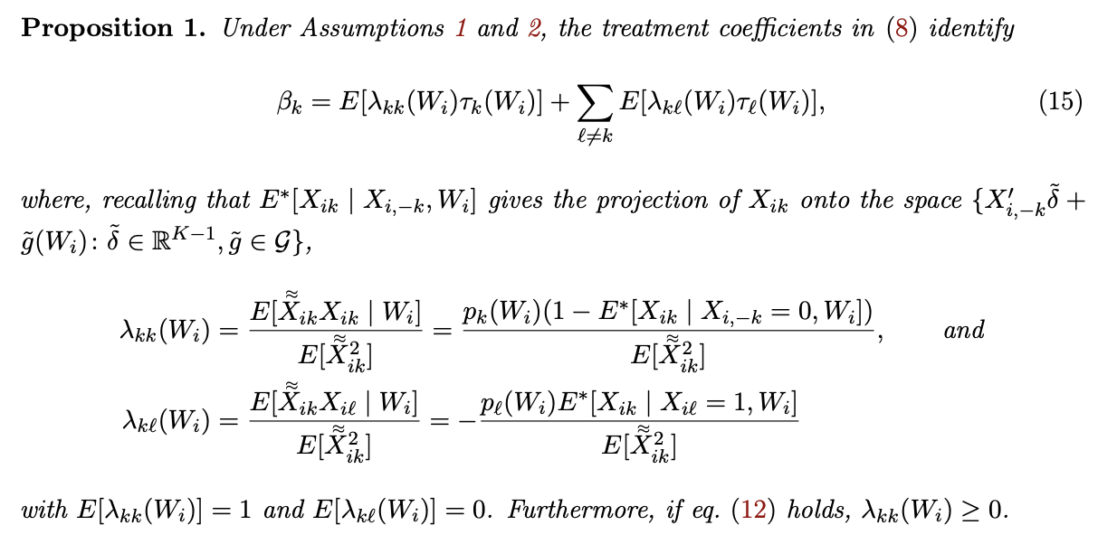
Unlike with a binary D, the estimates of $\beta_1$ and $\beta_2$ are not convex estimates of $\tau_1(w)$ and $\tau_2(w)$, but are instead contaminated by the other treatment effect:
\[\beta_{1}=E[\lambda_{11}(W_i)\tau_{1}(W_i)] + E[\lambda_{12}(W_i)\tau_{2}(W_i)]\]where $\lambda_{11}(W_i)$ can be shown to be non-negative and to average to one, similar to the $\phi$ weight in Angrist (1998). Thus, this second term is generally present: $\lambda_{12}(W_i)$ is generally non-zero, complicating the interpretation of $\beta_1$ by including the conditional effects of the other treatment $\tau_{2}(W_i)=E(Y_i(2)-Y_i(0)\mid W_i)$. [-3-] [-3-] See our paper for a fuller discussion of these exact terms.
Why does this contamination bias occur? Well, this comes back to the role of the controls $W$ in the regression. Controlling for $W$ in your regression is directly analogous to controlling for the pscore $p(W) = Pr(D=1 \vert W)$, thanks to the Frisch-Waugh-Lovell (FWL) theorem. But, now a given treatment ($X_{1}$) is a function of both the conditioning variables ($W$), and the other treatment ($X_2$)! That’s because if you get the first treatment, you can’t get the second treatment. Since we did not interact the treatments and $W$, the propensity score will not be correctly estimated – we will be measuring the “overall” propensity score, but not within a given strata.
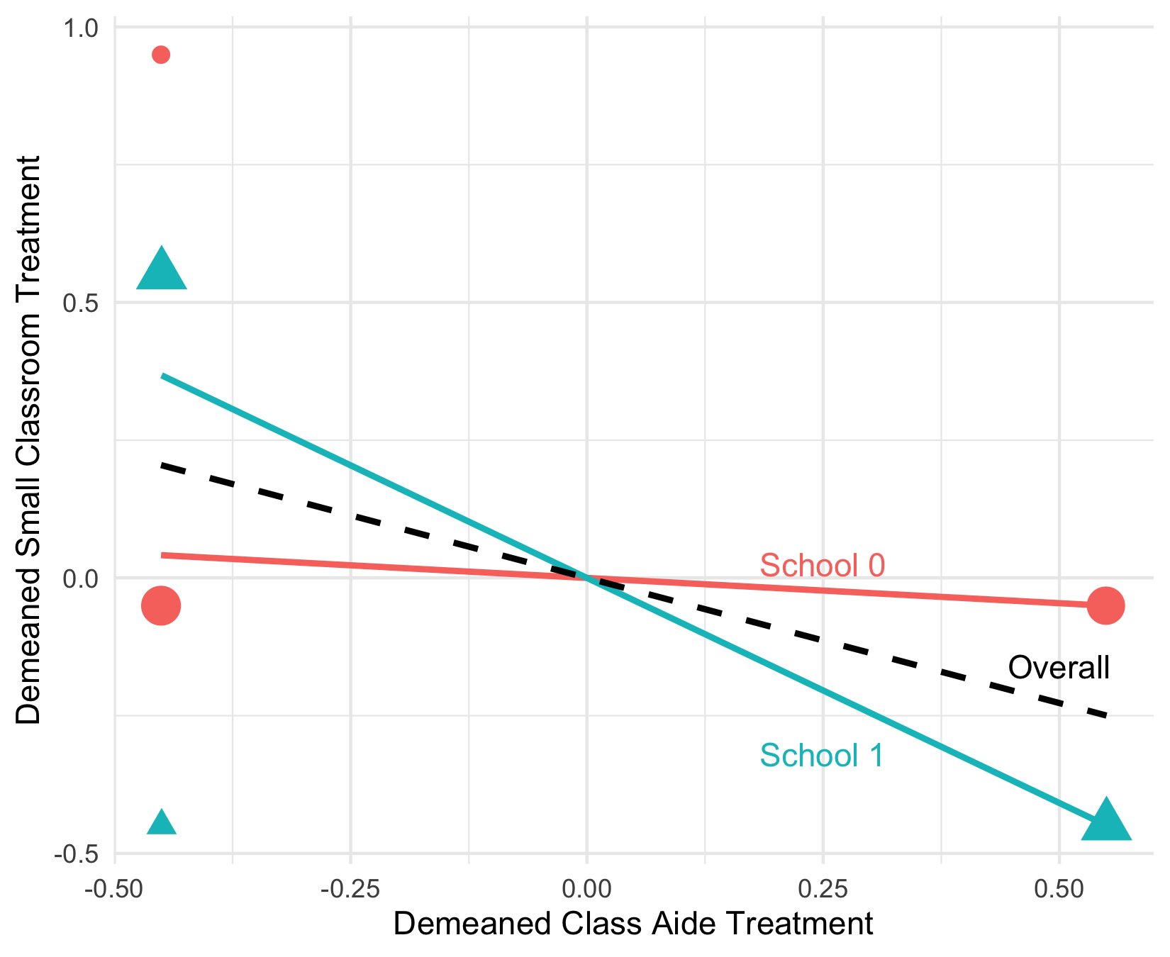
To give a stylized example, if schools vary in their treatment probabilities, the relationship between $\tilde{X}_{1} = X_1 - Pr(X_1 = 1 \vert W)$ and $\tilde{X}_2$ varies – in some schools, the two are highly negatively correlated (the blue line) while in others they are uncorrelated. Linear regression assumes the black line relationship, such that variation in $X_1$ after residualizing linearly for $X_2$ and $W$ tends to predict the $X_2$ treatment. This means that “treated” $X_1$ units are picking up “treated” $X_2$ units, thereby contaminating our estimates!
This is a broad result – with any multiple dependent treatments where controls are necessary – multi-armed stratified RCTs, Value-Added Models for teaching, or even group average differences (e.g. industry or race/ethnicity wage gaps) – this type of contamination bias can occur.
What drives the contamination bias?
What affects the magnitude and presence of the contamination bias?
- Heterogeneity in treatment effects
- Variation in pscores across controls (e.g. W is not correlated with D)
- Whether the variation in pscores covaries with the heterogeneity in treatments
Strikingly, this last case shows up in our empirical examples – it is interesting to think about heterogeneous TE and what exactly it is correlated with!
Another interesting feature of our main theorem is it highlights two conceptually distinct issues:
- whether there are negative weights on own treatment
- whether there is contamination bias.
As it turns out, negative weighting issues arise when the covariate specification in the regression is not flexible enough to correctly specify the propensity score. A simple example: two-way fixed effects cannot correctly approximate the “degenerate” propensity score from most DiD models (since there is no random variation in who is treated!) But the other issue of contamination bias also shows up in the differnece-in-difference literature, as remarked on by papers studying event study estimates in staggered events – when you are looking at multiple event horizons, these are multiple “treatments” which can contaminate one another.
Our paper highlights that the issues in DiD are a broader conceptual issue about
- the experimental design – having non-degenerate pscores will guarantee non-negative weights on own treatment
- the impact of multiple treatments in a regression model.
We flesh out the connection of our contamination bias paper to the new diff-in-diff lit in the Appendix B.
In the Appendix, we discuss four examples of DiD and how our main proposition nests these cases.
- a single intervention
- a staggered intervention with a single treatment
- a dynamic event study
- a single intervention period with multiple treatments
A single intervention is a la Card and Krueger’s famous minimum wage study, where there’s a single treatment intervention, and a treated and control group. In this case, there’s always positive weights and no bias! (A relief for many doing simple DiD!)
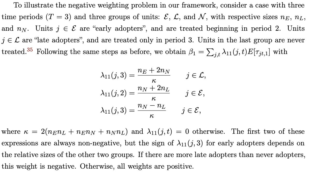
A staggered intervention with a single treatment is like the setting studied in De Chaisemartin and D’Haultfoeuille (2020) and Bacon-Goodman. In this case, you only have one treatment, so no contamination bias! But this is exactly the setting where these authors have shown negative weights can arise (but not always). In fact, we work out a special case with two interventions, three time periods, and one control group, and show that the negative weights only occur if there are more late adopters than never-adopters (the control):
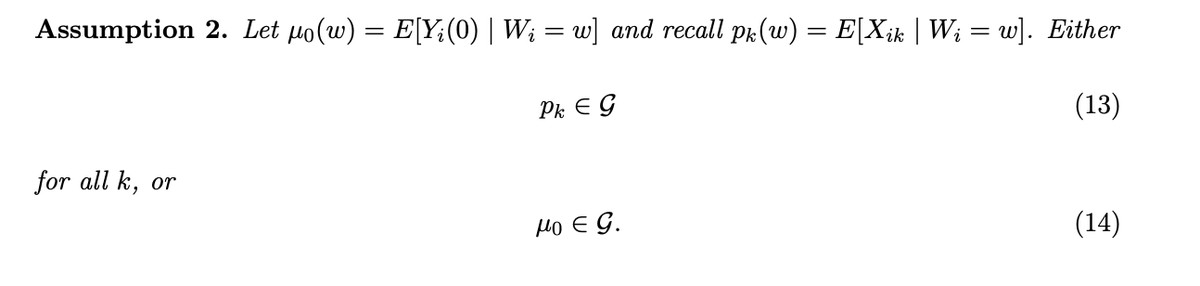
Importantly, we show in our paper that non-negative weights can’t be guaranteed because a “design-based” assumption doesn’t hold – treatment is not randomly assigned in most DiD designs. They are instead “model-based” – you assume that you correctly specify the control mean (Part (ii) of Assumption 2 above). [-4-] [-4-] The exception to this is in papers considering random assignment of timing of the DiD, as in Athey Imbens (2022)
Next, we consider a dynamic event study with staggered interventions. This setting is notationally a pain in the butt, but it is when you’re estimating leads and lags in a diff-in-diff. What does this do? Well, it creates many more dependent treatments you need to estimate! That implies that there will be contamination bias in our Proposition 1 – exactly in line with the existing DiD lit such as Sun and Abraham (2021) and Borusyak, Hull and Jaravel (2024).
We also work out a special case following our example with the static treatment, but now allowing for a pre-period effect (a pre-test) and a long-run effect. You can show that in this setting, if the groups are equally sized, the contamination bias for the pre-trend test is almost as big as the own treatment effect weights for the initial effect period:
\[\beta= \begin{pmatrix} \tau_{L, 1, -2}\\ 0\\ \tau_{E,3, 1}\\ \end{pmatrix}+\lambda_{E,0}\tau_{E,2,0}+\lambda_{L,0}\tau_{L,3,0},\]where \(\lambda_{E,0}= \frac{1}{\zeta } \begin{pmatrix} 3n_{L}n_{E}+n_{N}n_{E} \\ 3n_{L}n_{E}+2n_{N}n_{E} \\ -n_{L}n_{N} \end{pmatrix},\qquad \lambda_{L, 0}= \frac{1}{\zeta} \begin{pmatrix} -3n_{L}n_{E} -n_{N}n_{E} \\ 3n_{E}n_{L} + 2n_{N}n_{L} \\ n_{N}n_{L} \end{pmatrix},\) and \(\zeta=2(3n_{L}n_{E} + n_{E}n_{N}+n_{L}n_{N}).\)
To quote our appendix:
In other words, the estimand for the two-period-ahead anticipation effect $\beta_{1}$ equals the anticipation effect for late adopters in period 1 (this is the only group we ever observe two periods before treatment) plus a contamination bias term coming from the effect of the treatment on impact. Similarly, the estimand for the effect of the treatment one period since adoption, $\beta_{3}$, equals the effect for early adopters in period 3 (this is the only group we ever observe one period after treatment) plus a contamination bias term coming from the effect of the treatment on impact. The estimand for the effect of the treatment upon adoption, $\beta_{0}$, has no contamination bias, and equals a weighted average of the effect for early and late adopters. In this example, the own treatment weights are always positive, but the contamination weights can be large. For instance, with equal-sized groups, $\lambda_{E,0}=(2/5,1/2,-1/10)’$ and $\lambda_{L,0}=(-2/5,1/2,1/10)’$, so the contamination weights in the estimand $\beta_{1}$ are almost as large as the own treatment weights for $\beta_{2}$.
Finally, we consider a treatment design with multiple treatments and multiple transitions a la Hull (2018) and de Chaisemartin and D’Haultfoeuille (2023). Since there’s multiple treatments, and no random assignment, there is both the possibility of negative weights and there will be contamination bias. The negative weights are solved with random assignment, but not the contamination bias (that requires a different estimator).
Solutions
So how can you solve these issues? It turns out that Imbens and Wooldridge trick is by far the easiest solution, and works even with multiple treatments. But, overlap concerns tend to be more severe with multiple treatments, because some propensity scores necessarily become closer to zero or one as more treatment arms are added.
Can we generalize the logic of regression weighting without contamination bias? Yes! We consider solutions that generalize the intuition from a single binary treatment: place more weight on strata with evenly distributed treatments, less on strata with overlap problem:
\[\hat{\beta}_{\hat{\lambda}^{CW}, k}= \frac{1}{\sum_{i=1}^{N}\frac{\hat{\lambda}^{CW}(W_{i})}{\hat{p}_{k}(W_{i})}X_{ik}} \sum_{i=1}^{N}\frac{\hat{\lambda}^{CW}(W_{i})}{\hat{p}_{k}(W_{i})}X_{ik}Y_{i} - \frac{1}{\sum_{i=1}^{N}\frac{\hat{\lambda}^{CW}(W_{i})}{\hat{p}_{0}(W_{i})}X_{i0}} \sum_{i=1}^{N}\frac{\hat{\lambda}^{CW}(W_{i})}{\hat{p}_{0}(W_{i})}X_{i0}Y_{i}.\]When the treatment is binary and $\hat{p}$ is obtained via a linear regression, this weighted regression estimator coincides with the usual (unweighted) regression estimator that regresses $Y_{i}$ onto $D_{i}$ and $W_{i}$.
One very nice thing that comes from our results is that if you’re worried about contamination bias, and want a quick and dirty check – simply reduce your comparison down to a single treatment and control, and estimate the effects. This will satisfy the conditions of Angrist (1998) and will also be efficient in the class of estimators, as shown in our paper. If you find similar effects, you can be somewhat reassured that contamination bias is not driving the results.